
Build your collections Excel template, with the formulas ready
Two sheets, twenty-four columns and twelve formulas. That is everything a spreadsheet needs to track loans, calculate interest, show the balance and turn the late payers red. It is all below: copy it and keep it.
There is no file to download and no email to leave. The template is the structure, not the attachment: with the structure you fit it to how you collect; with an attachment you fight someone else’s.
What the sheet has to do to be worth anything
A template can stop at a list of names with an “owes” column. That is not a collections sheet yet: it is the notebook, on a screen. To actually replace the notebook it has to answer four questions without you doing any arithmetic.
How much each customer owes today, without subtracting payments by hand. How much they should already have paid at this point in the loan, which is not the same thing. How much came in today, to balance the cash before you sleep. And who is behind, so you know who to visit tomorrow.
The fourth is what separates a useful sheet from a pretty one. Arrears are not visible in the balance: a customer with a balance of $800 may be perfectly current and another with $180 may not have appeared in ten days. The only way to know is to compare what they have paid against what they should have paid by the days elapsed. That comparison is done with a formula, not from memory.
The rest of this page builds that sheet piece by piece. If you would rather understand the arithmetic of installments, capital and interest first, start with the guide to the loan amortization schedule and come back.
Sheet 1: “Loans”, one row per loan
Headers on row 1 and data from row 2. You only type columns A to G: the next ten calculate themselves. Paste each formula into row 2 and drag it down.
| Col. | Field | Formula (row 2) | What for |
|---|---|---|---|
| A | ID | you type it | L-001, L-002… It is the key that ties everything together. |
| B | Customer | you type it | Full name. |
| C | Route | you type it | Area or neighborhood. Used to filter the day’s visits. |
| D | Disbursement date | you type it | Short Date format. |
| E | Capital | you type it | What you handed over. |
| F | Interest | you type it | Percentage format. 20% is written 20%, not 0.2. |
| G | No. of installments | you type it | Daily, weekly or biweekly. |
| H | Total to repay | =E2*(1+F2) | Capital plus the loan’s interest. |
| I | Installment amount | =ROUNDUP(H2/G2,0) | Rounded up to the next whole unit. |
| J | Last installment | =H2-(G2-1)*I2 | Absorbs the rounding remainder. |
| K | Collected | =SUMIF(Payments!$B$2:$B$5000,$A2,Payments!$D$2:$D$5000) | Adds every payment with that ID. |
| L | Balance | =H2-K2 | What is left to collect. |
| M | Installments due | =MIN($G2,MAX(0,NETWORKDAYS.INTL($D2,TODAY(),"0000001")-1)) | Collection days elapsed, skipping Sundays. |
| N | Should have paid | =MIN($H2,$M2*$I2) | What ought to be collected by now. |
| O | Arrears | =MAX(0,$N2-$K2) | The arrears, in money. |
| P | Installments behind | =IF($I2=0,0,ROUNDDOWN($O2/$I2,0)) | The arrears, in installments. |
| Q | Status | =IF($L2<=0,"PAID",IF($O2<=0,"CURRENT",IF($P2<3,"LATE","ARREARS"))) | The portfolio traffic light. |
The ranges stop at row 500 on purpose. If you point at the whole column, Excel recalculates a million cells every time you record a payment and the sheet crawls on a phone. Raise the 500 when you need to.
The three money formulas, with numbers you can redo
A loan of $1,000 at 20%, over 26 daily installments. It is the typical case of daily collection Monday to Saturday for a month. Follow along with a calculator:
-
1. Total to repay — column H
=E2*(1+F2)1,000 × 1.20 = 1,200. The interest is applied to the capital once, which is how it is agreed on the street. If your rate is monthly and the term runs on, you need a different formula: the guide on how to calculate daily interest on a loan explains it.
-
2. Installment amount — column I
=ROUNDUP(H2/G2,0)1,200 ÷ 26 = 46.15. Nobody collects fifteen cents. The 0 rounds up to the next whole unit: 47. Up rather than down, because the remainder is deducted at the end and the customer is never charged more.
-
3. The last installment — column J
=H2-(G2-1)*I2The first 25 add up to 25 × 47 = 1,175. So the last one is 1,200 − 1,175 = 25. That difference is the most common argument in the trade: the customer who pays a little extra on the last visit and is left wondering. With this column, the sheet tells them beforehand.
Three short columns doing the work that otherwise ends up on a phone calculator in front of the customer. With them, two identical loans are calculated identically even if someone else sets them up.
Sheet 2: “Payments”, one row per payment
This is the mistake that sinks almost every template: recording payments on top of the loan, in “Payment 1”, “Payment 2”, “Payment 3” columns. When the customer pays twice in one day or overpays, the row runs out of space. Payments go on their own sheet, one under the other, forever.
| Col. | Field | Formula (row 2) | What for |
|---|---|---|---|
| A | Date | you type it | Ctrl + ; types today’s date without leaving the keyboard. |
| B | Loan ID | you type it | With a dropdown list: never typed by hand. |
| C | Customer | =IF($B2="","",VLOOKUP($B2,Loans!$A$2:$B$500,2,FALSE)) | Fills itself when you pick the ID. |
| D | Amount | you type it | The payment. This is typed and nothing else. |
| E | Payment method | you type it | Cash, bank transfer, wallet… |
| F | Collector | you type it | Needed to reconcile the cash per person. |
| G | Loan balance | =IF($B2="","",VLOOKUP($B2,Loans!$A$2:$L$500,12,FALSE)) | Careful: it shows today’s balance, not the balance on the payment day. |
Column B is never typed by hand. Select it, go to Data → Data Validation → Allow: List and set the source to =Loans!$A$2:$A$500. From then on the ID is picked from a dropdown and the most expensive error of all disappears at a stroke: a payment recorded against an ID that does not exist, which adds up nowhere and shows as missing money at close.
Let the sheet spot the arrears on its own
Column M counts how many collection days have passed since disbursement, skipping Sundays:
=MIN($G2,MAX(0,NETWORKDAYS.INTL($D2,TODAY(),"0000001")-1)) The seven digits of "0000001" are the days from Monday to Sunday, and the 1 marks the day you do not collect. You subtract 1 because no installment is collected on disbursement day. MIN stops the counter running past the last installment, and MAX prevents negative numbers if you record a loan with a future date.
With that, the rest follows. Example with the same $47 installment: 10 collection days have passed and the customer has paid 8 installments. They should have paid 10 × 47 = 470 and they have paid 8 × 47 = 376. The arrears are 94, that is 2 installments. Column Q flags it as LATE; on the third unpaid installment it becomes ARREARS.
Where to put the threshold is your call. Three installments works for daily collection. For weekly collection, a single overdue installment is already an urgent visit: change the 3 to a 1 in column Q. On when to call and what to say, the site has a guide to preventive collections that avoids reaching this column.
Conditional formatting: make the arrears visible from across the room
Select the range A2:Q500 and go to Home → Conditional Formatting → New Rule → Use a formula to determine which cells to format. Create one rule per line:
| Rule formula | Format and what for |
|---|---|
=$Q2="ARREARS" | Red fill. This is the row that should hurt when you open the file. |
=$Q2="LATE" | Amber fill. Still recoverable with a phone call. |
=$Q2="PAID" | Grey struck-through text. Stops getting in the way without being deleted. |
=$M2=$G2 | Thick border: every installment for that customer has now fallen due. |
What usually breaks this part is the dollar sign. $Q2 takes the dollar on the letter and not on the number. That way the rule always looks at column Q but moves down row by row and paints the whole record. If you write $Q$2, every row reads the first customer’s status and the whole sheet turns the same color.
The formula is written as if for the top-left cell of the selected range. Excel propagates it to the rest on its own. And add a data bar over column L: seeing the balance as a bar rather than a number shows in two seconds where the capital is concentrated.
The day’s cash close
Open a third sheet and paste these six formulas into loose cells. It is the dashboard you look at at nine in the evening before putting the money away.
| Indicator | Formula |
|---|---|
| Collected today | =SUMIF(Payments!$A$2:$A$5000,TODAY(),Payments!$D$2:$D$5000) |
| Collected today per collector | =SUMIFS(Payments!$D$2:$D$5000,Payments!$A$2:$A$5000,TODAY(),Payments!$F$2:$F$5000,"Luis") |
| Capital on the street | =SUM(Loans!$L$2:$L$500) |
| Portfolio in arrears | =SUMIF(Loans!$Q$2:$Q$500,"ARREARS",Loans!$L$2:$L$500) |
| Arrears ratio | =IF(SUM(Loans!$L$2:$L$500)=0,0,SUMIF(Loans!$Q$2:$Q$500,"ARREARS",Loans!$L$2:$L$500)/SUM(Loans!$L$2:$L$500)) |
| Customers in arrears | =COUNTIF(Loans!$Q$2:$Q$500,"ARREARS") |
Format the arrears ratio as a percentage. And before you finish: turn both sheets into a Table with Ctrl + T. The formulas copy themselves into every new row and that classic “I forgot to drag the formula”, which leaves customers out of the count, is over.
Where this template falls short
The sheet above works. We use it to explain and it does what it promises. But it would be dishonest to leave you with it without saying where it breaks, because it always breaks at the same six points. The contrast with the alternative is developed in Excel against a collections app.
It does not come on the route with you
Excel on a phone, standing up, with the sun in your eyes and the customer waiting, is useless. You end up writing in the notebook and typing the whole day into the sheet once you get home. In that transfer the payment nobody managed to write down disappears, and it does not surface until the customer complains with the receipt in hand.
It does not issue a receipt
The sheet calculates, but the customer leaves with no proof. And the proof is what ends the argument six months later, when somebody swears they already paid that installment.
It does not keep the past
The balance column always shows today’s balance. If you need to know where the loan stood on the 12th of last month, the sheet cannot tell you: the only way is to freeze values with Paste Special, and nobody does that every day.
It cannot take two hands at once
Two collectors cannot write in the same local file. If you put it in the cloud to share it, it stops working exactly where there is no signal — which is where collecting happens.
It does not warn you when you are wrong
If you type $500 instead of $50, the sheet accepts it and leaves the balance negative. And if you drag a formula one row short, a customer becomes invisible forever without anything turning red.
It breaks on refinancing
The model assumes a fixed installment. An extraordinary payment, a renegotiated term or a loan built on the previous balance force you to rewrite the row by hand, and that is where the audit trail is lost.
When to keep the sheet and when to let it go
Keep the template if you collect alone, if your portfolio fits in a notebook, if your customers do not ask for proof and if you genuinely sit down every night to type. In that case the sheet is free, it is yours and it depends on nobody. Change it when it gets in the way, not because someone told you spreadsheets are outdated.
Let it go the day a second collector joins, the day you start getting home too tired to type it up, or the first day a customer disputes a balance and you have nothing to answer with. Those three moments are what turn the sheet into a risk rather than a tool.
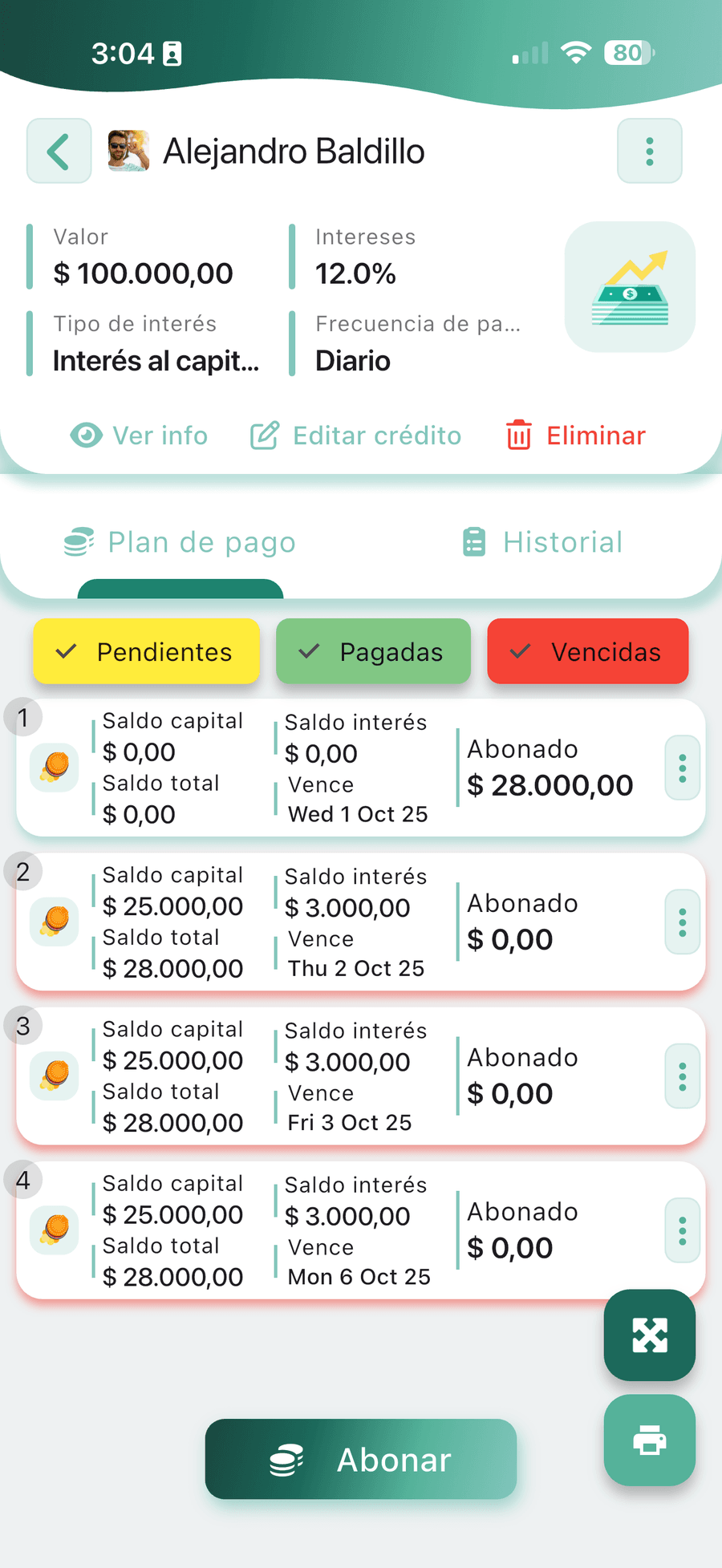
What comes after Excel is a collections platform that does on the street what the sheet only does at the table: record the payment at the customer’s door with no signal, print the receipt on a 58 or 80 mm Bluetooth printer and leave the balance updated on the spot. If your specific problem is the daily reconciliation, start with daily loan tracking; if it is the order of the visits, start with collection routes.
And you do not have to give up Excel for that. Reports download to Excel and CSV, so the sheet keeps existing for your accounting: what changes is who fills it in row by row. The free version goes up to 10 customers, with two loans each, which is enough to run part of the route in parallel and compare it against your template before moving anything. The limits of each plan are on plans and pricing.
Questions about the collections Excel template
What people ask while building their sheet, or while thinking about leaving it.
What does collections software give me that a spreadsheet does not?
Where do I download the collections Excel template?
Do the formulas work in Google Sheets?
How do I stop the template counting Sundays?
How do I stop someone deleting the formulas by accident?
How many customers can a collections Excel template take?
Can I move my Excel template into CobrApp without retyping everything?
$ 3,470.00 Balanced
What a route of 37 visits with 4 collectors brings in on one day, with the portfolio balanced at close.
When the sheet can no longer keep up
CobrApp calculates the interest when the loan is created, prints the receipt over Bluetooth and leaves the balance updated on the spot. It works with no internet and exports to Excel when you need it.
CobrApp does not grant credit or lend money. It is a technology platform for collections management and portfolio control of loans issued by third parties.